
Control Systems Part 1: Introduction To Control Systems & Controllers
Effectively tuned control loops provide for more efficient and safer operation. After process startup, there are various techniques available for tuning controllers ranging from trial and error methods to mathematically sophisticated programs. Few options are available for tuning loops prior to startup. Many control systems are started with the manufacturer’s default tuning parameters. This series of GATEKEEPERS will provide methods for using readily available process design data for determining effective tuning parameters before startup.
The Operation of the Controller
Figure 1 shows a simple level control loop. The level transmitter (LT), measures the level and sends a signal proportional to the vessel level to the level controller (LC). The controller instructs the level control valve (LCV) to open or close as needed to keep the level at or near the set point.

In this series of GATEKEEPERS, we will be mainly concerned with the operation of the controller. Figure 2 illustrates the operation of the transmitter and controller.

The transmitter (XT) accepts the process variable (level in ft) and converts it into a process variable signal (PV) expressed as a fraction of the transmitter range. PV has a value between 0 and 1. For the system shown in Figure 1, the transmitter range will be 0 to 6 ft. Note that the vessel itself has a diameter greater than 6 ft, but the level instrument does not span the entire diameter. If the vessel is operating at the normal liquid level of 3 ft, then the XT signal will be 3/6 = 0.5.
The XT output (PV) is fed to the Controller, where it is compared to the Set Point (SP), also a 0-1 signal, to generate an error signal (e). Finally, a control algorithm (ALG) is applied to generate a controller output signal; Controller Output (CO) = Valve Position (Pos). We will call this signal Pos, because that signal instructs the valve to seek that position.
Note that signals can be filtered to reduce noise at both the controller (Tf2) and transmitter (Tf1) found in Figure 2. The application of filters is not considered in this GATEKEEPER series.
PID Controller
The most common controller type is a PID controller. A PID controller has three functions:
Proportional Action: Takes action proportional to the error; small error yields minor valve movement, large error yields large valve movement.
Integral Action: Takes action proportional to the integral of the error. Here a small error that has existed for a long time will generate a large valve movement.
Derivative Action: Takes action proportional to the derivative of the error or process variable. A rapidly changing error generates a large valve movement.
The most common PID algorithms are Parallel, Ideal and Series. The Ideal algorithm shown below is used for the remainder of this GATEKEEPER series:

If there is no error (steady state operation) the position of the control valve will be Posss. The right side of the equation above will equal zero. If there is an error (level is different than the set point) then the algorithm will instruct the valve to move to a new Pos. As noted above, the response of the valve is based on three tuning parameters. The main parameter is controller gain (Kp). Pos changes in direct proportion to the value of Kp. The larger Kp is, the larger the valve movement.
The second important term is referred to as the integral time or reset time (Ti). In this algorithm, Kp/Ti acts on the integral of the error. Note that if the constant error exists for the time period Ti, then the gain, Kp, is reproduced by the integral action. The third tuning parameter, derivative time (Td), acts on the derivative of the error (rate of change).
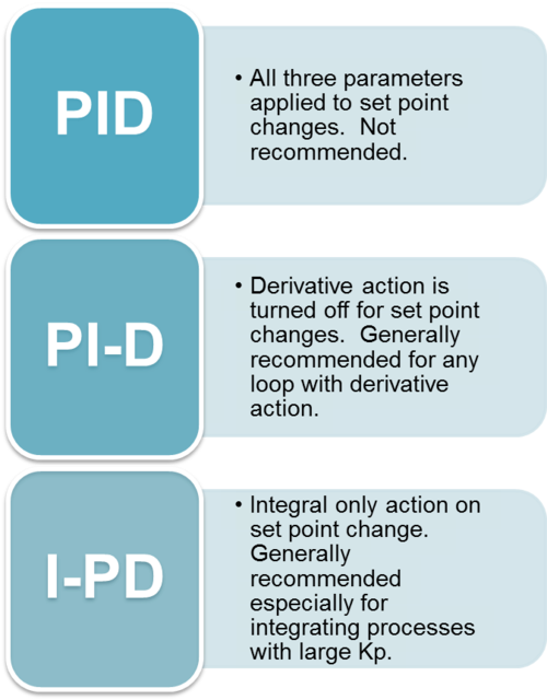
Note that the PID algorithm can be applied to behave differently depending on whether the error is caused by a set point change or a process demand. Table 1 shows the typical options. In particular, we would generally not want derivative action applied to a set point change.

Example Calculation
The vessel shown in Figure 1 has level bridle that is 6 ft tall.
Transmitter (XT) Range = 0 to 6 ft
Set Point (SP) = Normal Liquid Level (NLL) = 3 ft
Gain (Kp) = 2,
No integral action (Ti very large) and No derivative action (Td = 0).
Valve position is 50% open at normal flowrate and level.
What will the valve position (Pos) be when the level is 2 ft?
SP = 3 ft = 3/6 = 0.5
At 2 ft level the error, e = -1 ft = -1/6 = -0.17
Since we have only proportional action, the control algorithm is:
Pos = Posss + Kp(e)
Pos = 0.5 + 2(-0.17) = 0.16
So, if the level drops 1 ft (from 3 ft to 2 ft), the valve will move from 50% open to 16% open in an effort to build the level back to normal.
Next in the Series
In the next GATEKEEPER, the focus will shift to discussing how to determine effective values for the tuning parameters Kp and Ti. Tuning parameters will be based on a simple dynamic model using three parameters:
Process Gain (PG),
System Time Constant or Lag (Tc), and
Dead Time (DT). It is important not to confuse Dead Time with Derivative Time (Td).