
Control Systems Part 2: Introduction To System Dynamics - Tuning Controllers For Initial Startup
This is part two of the GATEKEEPER series on control systems tuning. To effectively tune a control loop, there needs to be an understanding about the dynamics of the system. The intention of this GATEKEEPER is not to provide a detailed review, but to provide an 80/20 solution.
For most loops we can describe system dynamics adequately for pre-startup tuning with three parameters:
Process Gain, PG.
System Time Constant or Lag, TC.
Dead time, DT (not to be confused with derivative time, Td).


Self-Regulating vs. Integrating Process
A system responds to a disturbance in one of two ways; either by self-regulating, or by integrating. In a self-regulating process, the process variable will change to a new steady state without any control action (See Figure 1). Vessel pressure control is an example. If you close the control valve a little, the pressure will increase some and then settle out at a new steady state.
In an integrating process, on the other hand, the process variable does not reach a new steady state (See Figure 2). Level control is an example. If you close a level control valve a little, the level climbs until the vessel fills/overflows.
Process Gain
Process gain, PG, is a measure of how much the process variable changes for a given change in valve position. For a self-regulating loop, PG is the change in process variable divided by the change in valve position. For an integrating loop, the PG is the slope of the process variable (with units in percent per second), divided by the change in valve position. In this instance, the process demand change causes unlimited process variable change.
Note that PG is a function of valve size and transmitter span. For example, doubling the valve size will double the PG. Doubling the transmitter span will result in the PG being cut in half.
System Time Constant (TC) & Lag
In a self-regulating process, it takes time to go from one steady state condition to another after a valve position change. This lag is measured by its time constant (TC), which is the time taken for the process variable to reach 63.2% of the new steady state (see Figure 3).
Since an integrating process does not reach a new steady state, a different definition is required. For this series, we will use the usable residence time in a vessel, such as the time between Normal Liquid Level (NLL) and Level Switch Low (LSL), as a representative time constant.
Sources of lag include:
Process lag (self-regulating process). For example, the time taken for vessel pressure to move from one steady state to another.
Actuator/Positioner Lag (time to pressure actuator).
Valve stroke time.
Instrument lag. For example, the time taken for a thermocouple reading to adjust to a temperature change.
Transmitter and Controller Filters.
Heat exchanger thermal mass.
Fluid inertia.
Rotating equipment inertia.


Figure 4 shows a simple way to estimate the time constant for a self-regulating process:
Determine the new steady state,
Determine the initial rate of change,
Find the intersection of the two lines.
Dead Time, DT
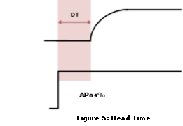
Dead time is the time between a disturbance and when the process variable actually begins to move (see Figure 5). Sources of dead time include:
Residence time in a plug-flow system, such as when a measurement is in a pipe some distance from the control point.
Measuring instrument dead time.
Valve stick (friction prevents it from moving until sufficient force is added).
Valve hysteresis (slop in linkage).
Actuator/Positioner dead time (time to build actuator pressure sufficient to move the valve).
Controller scanning time.


Ultimate Gain (Upper bound on Gain)
A good place to start a tuning discussion is to identify the upper bound on the gain, Kp. All loops have some dead time and any loop with dead time can be made unstable by giving it too high a gain.
There is a gain that will cause a constant cycling (see Figure 6). That gain is called the ultimate gain, UG. The UG is valuable as it sets the upper bound on the gain. As a general rule, the gain may be set at less than half the UG. At Kp = UG/2, expect approximately quarter amplitude dampening (red line in Figure 6), which is too fast for many industrial loops.
Estimating the Ultimate Gain
After startup, it is possible to determine the UG by gradually adjusting the gain until the process cycles. Prior to startup,UG can be estimated via the plot in Figure 7. All the inputs to the plot can be calculated from available process data or estimated from knowledge of the process and control system. As the GATEKEEPER series continues, focus will be dedicated to working examples and providing tuning rules based on the Figure 7 ultimate gain plot.