
Wax Management Strategy Part 2: Wax Deposition Modeling
Wax deposition modeling is essential to estimate the wax deposit thickness over time in support of wax management strategy development for susceptible systems. The objective of this GATEKEEPER is to provide a high-level overview of the model commonly used in the industry to estimate the wax deposition.
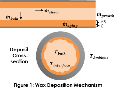
Several mechanisms are considered when calculating wax deposition. These include wax mass transfer from the stream (m ̇_bulk), wax mass rate removed or prevented by shear (m ̇_shear), mass transfer in the deposit (m ̇_aging) and mass rate for the deposit growth (m ̇_growth). The illustration of these mechanisms are depicted in Figure 1. The methodology introduced in this publication is incorporated in GATE’s in-house wax deposition simulator, Pwax. The step-by-step calculation of wax deposition modeling can be found below.
STEP 1: OBTAIN STREAM’S HYDRODYNAMIC PARAMETERS
Wax deposition is a thermal-hydraulic dependent phenomenon. Numerous hydrodynamic and thermal parameters such as in-situ flow rates of oil and gas, liquid holdup, flow pattern, flow regime, pressure and temperature are needed in this analysis. Multiphase thermo-hydraulic simulators can be utilized to provide these parameters. Since the wax deposit reduces the effective diameter of the pipe and acts as an insulator, thermal-hydraulic parameters need to be recalculated as the deposit grows. Pressure and temperature measurement in the flowline can be used in lieu of simulation results in the actual field cases or to calibrate the hydrodynamic model.
STEP 2 : DETERMINE THE TEMPERATURE AT STREAM-DEPOSIT INTERFACE (T_INTERFACE)
The temperature at the stream-deposit interface (T_interface) needs to be calculated to determine the wax concentration at the interface. This dictates the driving force of wax deposition, the wax concentration radial gradient. A heat transfer model with overall heat transfer coefficient incorporating both convective heat transfer film coefficient in the stream and conductive heat transfer coefficient of the wax deposit (k_deposit) is required. Convective heat transfer film coefficient can be estimated using the Nusselt number (N_Nu) calculated by the Sieder-Tate Correlation (1936) for turbulent flow while the conductive heat transfer coefficient of the deposit is calculated using the Maxwell Equation (1959).
STEP 3 : CALCULATE WAX MASS TRANSFER FROM THE STREAM (M ̇_BULK)
The m ̇_bulk model predicts the wax mass rate coming out from the stream due to radial wax concentration gradient at the deposit-stream interface. The two industry standard diffusion models in estimating m ̇_bulk are the equilibrium and the heat analogy model. Pwax uses both models while OLGA® Wax utilizes the later (4). Both models require Diffusion Coefficient (D_wo) and wax solubility curves (Figure 3). D_wo is calculated using the Wilke-Chang correlation (1955) to be consistent with the Matzain (1999) deposition model discussed in Step 4. An alternative model to predict D_wo is the Hayduk-Minhas correlation (1982). The wax solubility curve can be obtained through crude oil composition modeling or lab testing (e.g. High Temperature Gas Chromatography measurements).
STEP 4: CALCULATE WAX MASS RATE CONTRIBUTES TO DEPOSIT GROWTH (M ̇_GROWTH)
Some fractions of m ̇_bulk may not contribute to the deposit growth due to the complex deposit aging mechanism and shear effects. Aging in the deposit occurs due to the counter-diffusion of trapped oil in the existing deposit to the stream and wax diffusion through the existing deposit layer. This mechanism leads to a harder deposit over time. A model developed to take these effects into account was introduced by Singh et al. (2000).
Shear induced by the flow may remove some portion of the existing deposit or prevent wax deposition to some extent. The actual physical mechanism on shear effects is not well understood and is subject to further research. A semi-empirical model to cover these phenomena as well as any positive deposition rate not accounted for by the diffusion constant (D_wo) was developed by Matzain et al. (1999). The Matzain diffusion model is incorporated in both PwaxTM and OLGA® Wax (4).
It also covers the effects of flow regime and flow pattern (for wax deposition under multiphase flow). Using the conservation of mass, wax mass rate contribution to deposit growth can be calculated:

STEP 5 : CALCULATE THE DEPOSITION RATE
m ̇_bulk calculated in Step 4 is used to determine the deposit thicakness growth rate at a given time. Average wax density (ρ_wax) and trapped oil volume fraction in the deposit (F_o) are required to perform this calculation.

The deposition growth rate varies with time due to several factors:
As the incipient deposit grows thicker, it acts as an insulator and therefore increasing T_interface and reducing the wax deposition driving force.
The wax deposit reduces the effective diameter of the pipe, resulting in a higher stream velocity. This leads to a more turbulent flow, so a higher shear force on the deposit is expected. It may also affect the flow pattern when the system is operating under multi-phase conditions.
The effective diameter reduction caused by the wax deposit also introduces additional pressure drop which may cause backpressure to the production wells and decrease the production flowrate.
STEP 6 : CALCULATE THE WAX THICKNESS OVER TIME , Δ(T)
The deposit thickness over time can be determined by performing progressive calculation of

by repeating Step 1-5 every ∆t and integrating

in respect to time as follows:

SINGLE WELL TIEBACK EXAMPLE CASE
The methodology above can be applied to the hypothetical single well tieback case, introduced in Wax Management Strategy Part 1: Establishing Initial Wax Risk and shown in Figure 2. The wax solubility curve, which was previously generated by DSC analysis during the initial wax risk assessment, is shown in Figure 3.


Results from GATE PrhoTM are shown in Figure 4. These results were used as inputs to determine wax deposition thickness as a function of time in the flowline. Initial results showed that a location 14 miles away from the wellhead exhibited an elevated deposition risk.
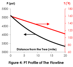
At this location, GATE PrhoTM predicts a single phase oil flow with 4,370 psi pressure and 92˚F temperature during the initial flowrate condition.
Using this hydrodynamic data and the wax solubility shown in Figure 3, Pwax predicts a substantial risk for wax deposition in the flowline – approximately 0.75” per year. The simulation results can be found in Figure 5.

The wax deposition has the following consequences:
Reduction of the effective diameter of the pipe
Introduction of additional pressure drop which may cause backpressure to the production wells and decrease the production flowrate.
Possible flow pattern disruption when the system is operating under multi-phase conditions.
Development of a wax mitigation strategy is now a necessary requirement for the hypothetical production pathway. The deposit thickness over time prediction will be used as an input in developing wax deposition prevention and remediation activities such as: determining pigging frequency, chemical inhibition/dissolution viability, and insulation effectiveness. All of these activities must be carefully considered and used where appropriate to design a robust, viable wax management strategy. This is the subject of the next GATEKEEPER in this series.

REFERENCES
Matzain, A. 1999. Multiphase Flow Paraffin Deposition Modeling. Ph.D Dissertation, The University of Tulsa, Tulsa, OK
Singh, P., Venkatesan, R., Fogler, H.S. and Nagarajan, N. 2000. Formation and Aging of Incipient Thin Film Wax-Oil Gels. AIChE J. 46 (5): 1059 - 1074.
Wilke, C.R. and Chang, P. 1955. Correlation of Diffusion Coefficientin Dilute Solution s. AIChE J. 1 (2): 264-270.
https://www.software.slb.com/products/olga/olga-solids-management/wax